Neural Surface Potentials for Fast Flow Approximation

Abstract

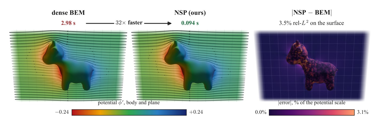
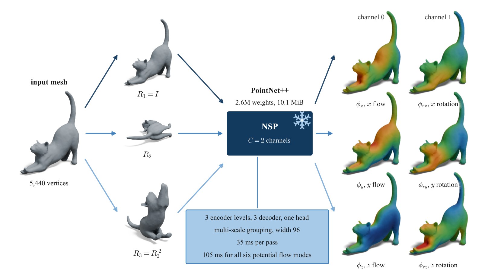
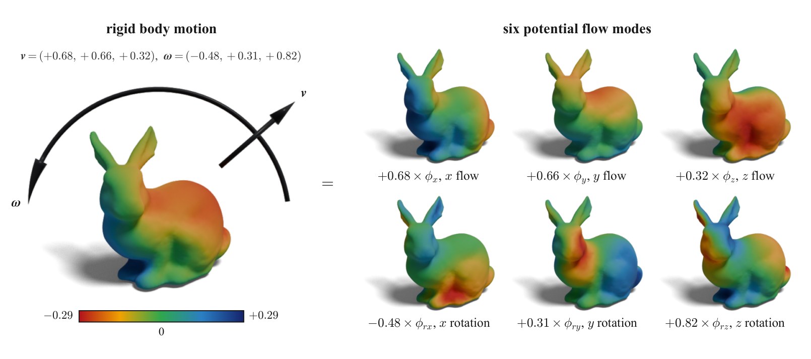
The potential flow around a rigid body moving through an ideal fluid is determined by six harmonic potentials on its surface, one per rigid degree of freedom. Computing them requires a boundary-integral solve per shape, which has to be repeated whenever the body deforms. We present Neural Surface Potentials (NSP), a feed-forward network that predicts all six potentials from a closed triangle mesh without per-mesh precomputation. Two properties of the problem shape the method. By linearity, the six fields give the potential of any rigid motion as a weighted sum. By rotation equivariance, a network with one translational and one rotational output recovers all six fields from three passes on rotated copies of the mesh, and rotation augmentation comes with exact labels at no cost. Trained on about ten thousand shapes, NSP reaches median field errors of 4.0 to 6.7 % on validation shapes and 5.3 to 10.2 % on a harder held-out test set, and it recovers the 6×6 added-mass tensor to a median error of 1.05 % and 1.58 %. All six modes take 105 ms on a mesh of about 6 000 vertices, 34 times faster than the double-precision dense solve that produced the training labels. A simple shape descriptor, the isoperimetric ratio, predicts on which meshes the network is least accurate.

Method

NSP is a PointNet++ encoder-decoder that reads the vertices of a closed triangle mesh, with their positions and normals in a canonical frame, and returns the potential at every vertex without any precomputation. The problem is linear in its boundary data, so the six Kirchhoff potentials, one per rigid degree of freedom, give the potential of any rigid motion as a weighted sum. The problem also commutes with rotations, so a network that predicts one translational and one rotational potential recovers all six from three passes on rotated copies of the mesh. The same identity turns rotation augmentation into exactly labelled training data by randomizing the orientation. The training labels come from a dense boundary-element solve on 10 418 shapes from Thingi10K and Manifold40.

Inference on an unseen body. The mesh is turned by the cyclic rotation x → z → y → x and the same network runs on each copy. Channel 0 returns a translational potential and channel 1 a rotational one, so three passes give all six modes.

Six fields describe every rigid motion. The potential of a body that translates and rotates at once is the weighted sum of the six predicted modes; it differs from a dense solve of the combined problem by 4.07 %. Each small panel has its own colour scale.

Results

Live inference on a deforming body

A body bends and the network predicts its potential φ_x for every pose.

BibTeX

@misc{padilla2026nsp,
  title        = {Neural Surface Potentials for Fast Flow Approximation},
  author       = {Padilla, Marcel},
  year         = {2026},
  howpublished = {Preprint, ETH Z\"urich},
  url          = {https://marcelpadilla.com/Neural_Surface_Potential/}
}